A bioinformatic study of Arthritic B Cells

Introduction
In inflammatory arthritis, immune cells are ironic drivers of the disease. B cells in particular play a pivotal role by producing autoantibodies that target joint tissues, forming immune complexes that trigger inflammation, and secreting pro-inflammatory cytokines. Their interaction with T cells further encourage these cycles of chronic inflammation and joint destruction. As a result, targeting B cells has emerged as a promising therapeutic strategy in RA, with drugs like rituximab showing efficacy in reducing inflammation and preventing joint damage.
Recently, advancements in single-cell RNA sequencing (scRNA-seq) have changed our understanding of this cellular heterogeneity and gene expression at the individual cell level. If you have ever wondered how our body’s cells differ from one another at the genetic level, in this project we will conduct a comprehensive analysis of Arthritic B cell scRNA-seq data using the Seurat package in R, offering insights that could deepen our understanding of inflammatory arthritis.
Normalizing and Scaling
Before we dive into the nitty-gritty, let’s lay the groundwork. First, we’ll explore the data and focus on B cells, followed by the essential steps of normalizing and scaling. Normalization ensures that cells have comparable gene expression profiles, regardless of their size, while scaling prevents genes with higher expression values from overshadowing others. These steps are crucial for downstream analysis, allowing us to focus on potential biologically relevant variations.
NB: Some pre-steps were already performed on the “mother” dataset.
#libraries
library(Seurat)
library(patchwork)
library(dplyr)
library(ggplot2)

#normalizing and scaling----------------------------------------------
bcells <- readRDS("bcells_p.rds")
bcells <- NormalizeData(bcells)
bcells <- FindVariableFeatures(bcells , selection.method = "vst", nfeatures = 2000)

# Identify the 10 most highly variable genes
top10 <- head(VariableFeatures(bcells ), 10)
top10

bcells <- ScaleData(bcells)

bcells <- RunPCA(bcells)
#Think of PCA as viewing a 4D (a higher dimension) object in 2D (lower dimension). PCA helps organize cells based on how similar their genes are, capturing the most important patterns of variations in data, usually by the first few components.
ElbowPlot(bcells)
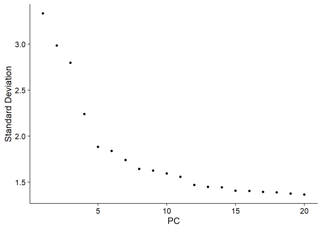
#the elbow plot helps to pick the components important for clustering.
Clustering
Moving on to clustering, an important step for identifying groups of cells with similar genetic expression. This provides biological insight into the inherent organization of the cell population and helps with quality control by revealing outliers or misclassified cells.
bcells <- FindNeighbors(bcells, dims = 1:15)
bcells <- FindClusters(bcells, resolution = 0.2)
# Look at cluster IDs of the first 5 cells
head(Idents(bcells), 5)


bcells <- RunUMAP(bcells, dims = 1:15)
gridExtra::grid.arrange(
  DimPlot(bcells, reduction = "umap"),
  DimPlot(bcells, group.by = "NUMBER"),
ncol=2
)
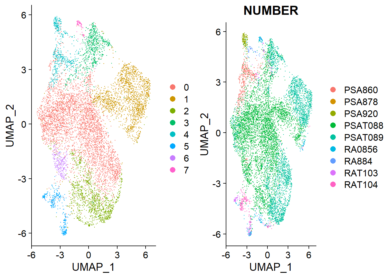 In this case, we have 8 clusters with no clearly defined groups that look suspiciously similar to the b cells grouped by patient number, which suggests we have to refine data preprocessing steps.
Integration and Regularization
Integration is key to avoid biological differences from patients. By integrating data, we leave behind patient variation, resulting in clusters that better represent the B-cell population.
bcells.list <- SplitObject(bcells, split.by = "NUMBER")
bcells.list

#integration problems, this patients dont have enough b cells
dataset_to_exclude <- c("PSA878", "RA884")

bcells.list <- bcells.list[setdiff(names(bcells.list), dataset_to_exclude )]

# Normalize and run dimensionality reduction on each dataset separately
bcells.list  <- lapply(X = bcells.list , FUN = function(x) {
  x <- NormalizeData(x)
  x <- FindVariableFeatures(x, selection.method = "vst", nfeatures = 2000)
})

# select features that are repeatedly variable across datasets for integration
features <- SelectIntegrationFeatures(object.list = bcells.list)

bcells.anchors <- FindIntegrationAnchors(object.list = bcells.list, anchor.features = features)
 #View(bcells.anchors)

bcells_int<- IntegrateData(anchorset = bcells.anchors)

#saveRDS(bcells_int, "bcells_int.RDS")

DefaultAssay(bcells_int) <- "integrated"

bcells_int<- ScaleData(bcells_int)
bcells_int <- RunPCA(bcells_int , verbose = FALSE)
bcells_int  <- FindNeighbors(bcells_int , reduction = "pca", dims = 1:15)
bcells_int <- FindClusters(bcells_int, resolution = 0.5)
bcells_int <- RunUMAP(bcells_int , reduction = "pca", dims = 1:15, verbose = FALSE)


gridExtra::grid.arrange(
  DimPlot(bcells_int, reduction = "umap"),
  DimPlot(bcells_int,group.by = "NUMBER"),
ncol=2
)
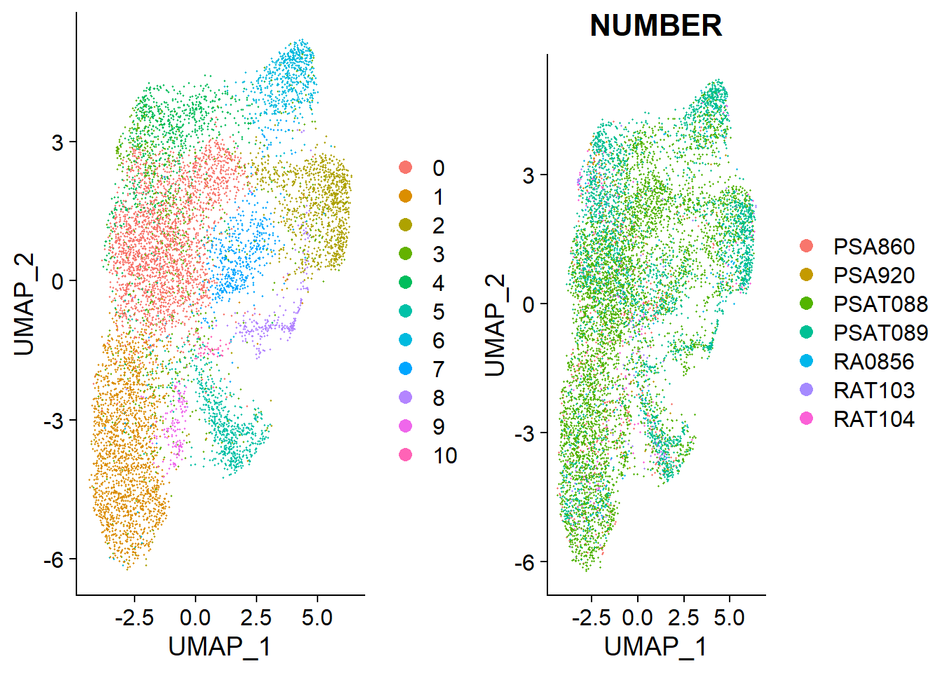
These new clusters have left behind patient variation and hence the clusters are better representative of the b-cell population.
# find markers for every cluster compared to all remaining cells, report only the positive ones

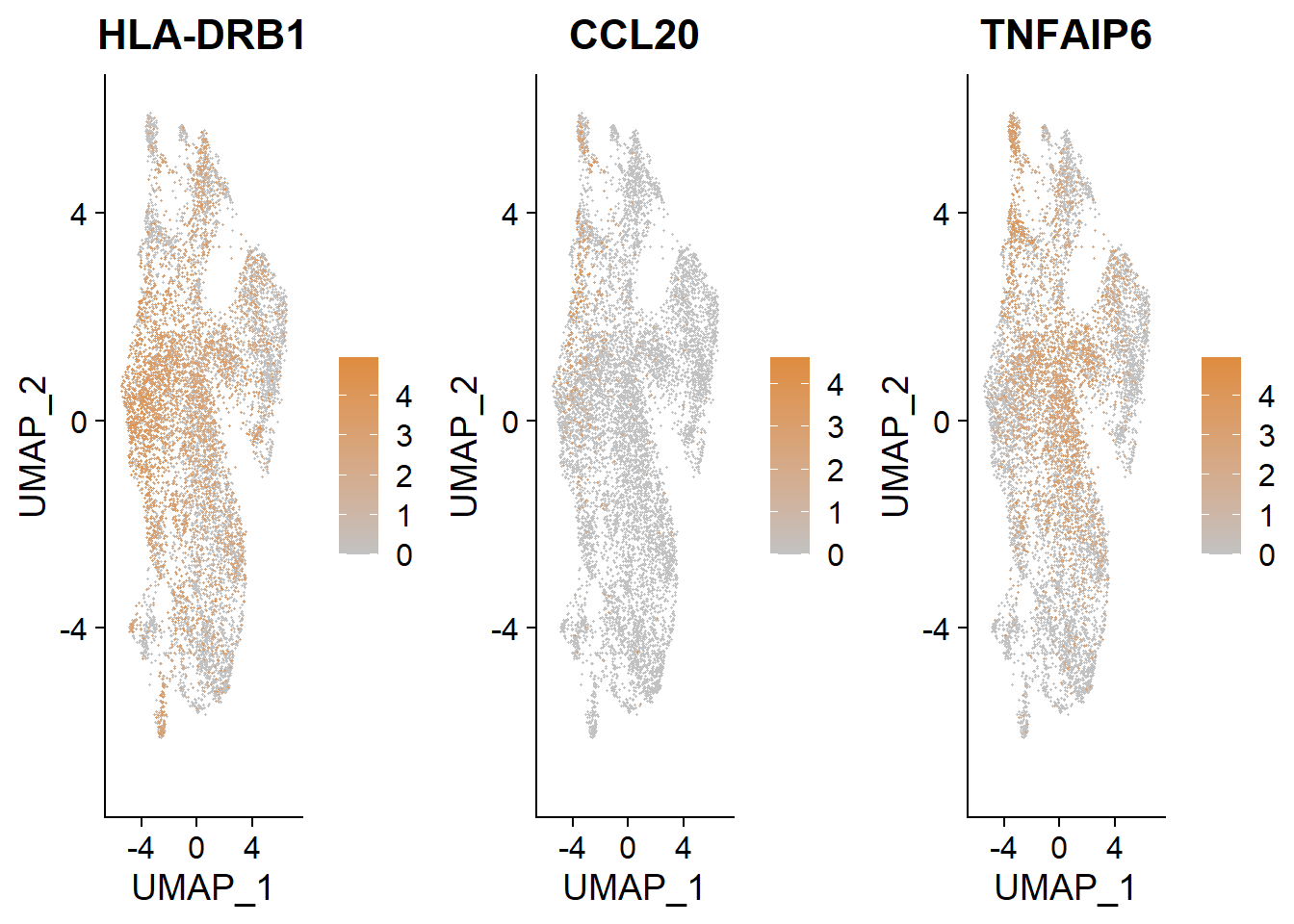
bcells.markers <- FindAllMarkers(bcells, only.pos = TRUE, min.pct = 0.25, logfc.threshold = 0.25)
bcells.markers %>%
    group_by(cluster) %>%
    slice_max(n = 2, order_by = avg_log2FC)


gridExtra::grid.arrange(
  FeaturePlot(bcells, features = "HLA-DRB1", order = TRUE, cols = c("#C2C2C2", "#DE8C3F")),
  FeaturePlot(bcells, features = "CCL20", order = TRUE,   cols = c("#C2C2C2", "#DE8C3F")),
  FeaturePlot(bcells, features = "TNFAIP6", order = TRUE,   cols = c("#C2C2C2", "#DE8C3F")),
  ncol = 3
)
Trajectory
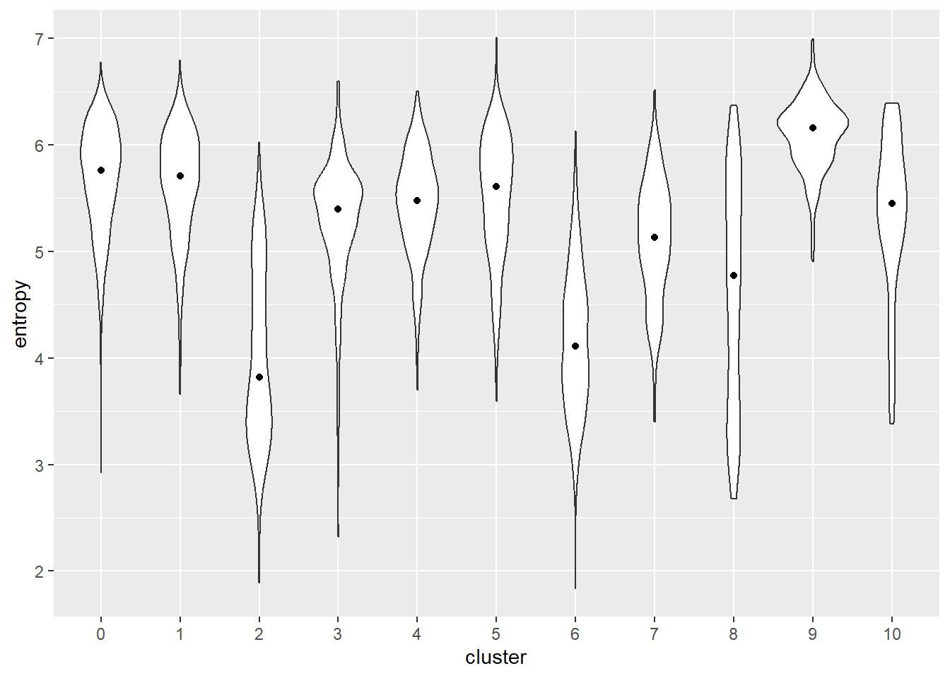
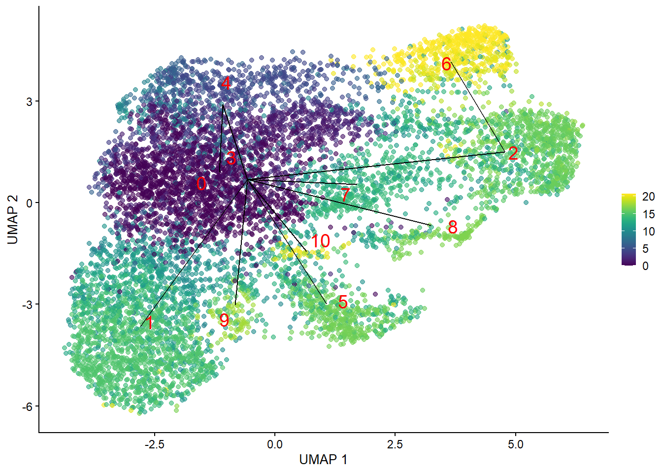
In simple terms, this is the path of cells to different states. It measures the continuum of dynamic changes in cellular state in pseudotime (we are imagining the distance between cells as time).The start of the trajectory is important here because this gives information on the cellular state of the b cells which in turn provides a window into the cellular processes that might be going on in these cells. For example what cell cycle, immune activation state the clustered cells might be in. Additionally, tests like entropy and the elbow plot provide insights into where the start of a trajectory might be.
bcells_sce =  as.SingleCellExperiment(bcells_int, assay = "SCT")

library(TSCAN)
entropy <- perCellEntropy(bcells_sce)
colLabels(bcells_sce) = bcells_int$seurat_clusters

ent.data <- data.frame(cluster=colLabels(bcells_sce), entropy=entropy)
ggplot(ent.data, aes(x=cluster, y=entropy)) +
    geom_violin() +
    stat_summary(fun=median, geom="point")
library(scater)
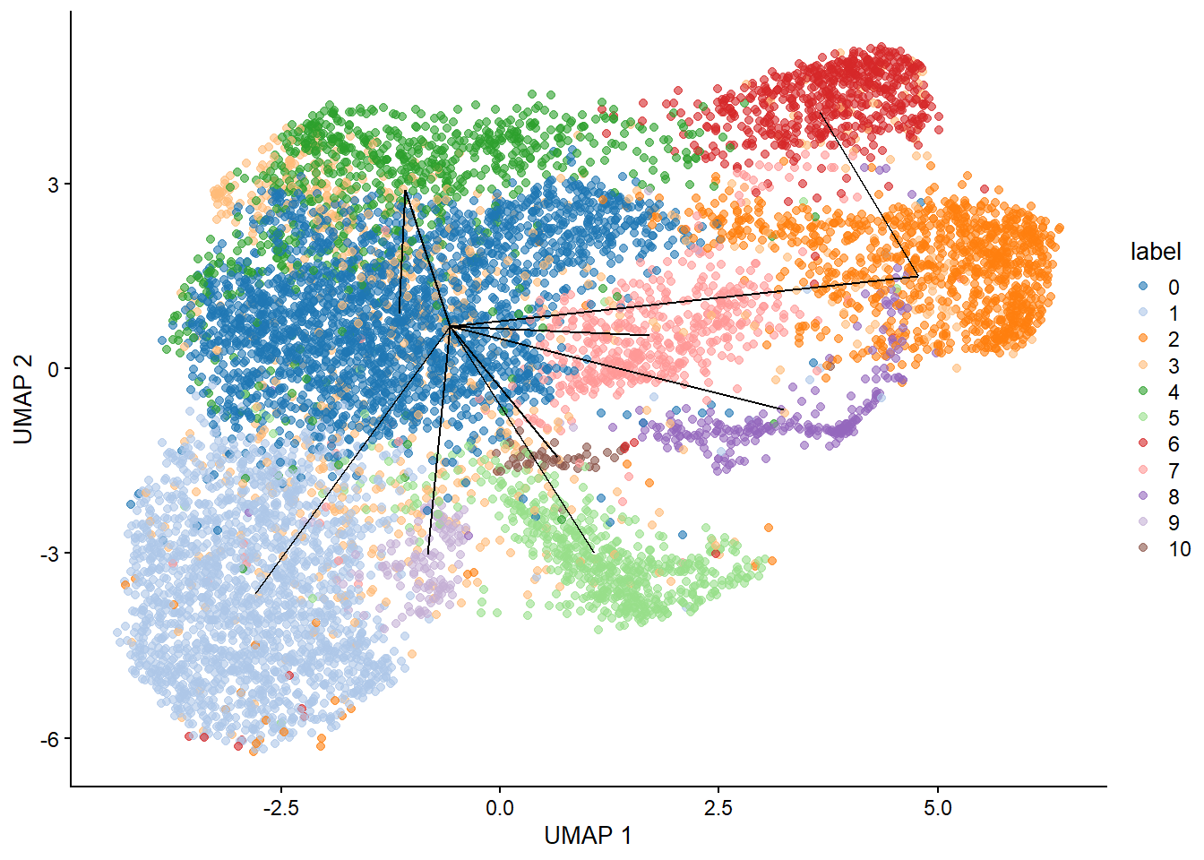
by.cluster <- aggregateAcrossCells(bcells_sce, ids=colLabels(bcells_sce))
centroids <- reducedDim(by.cluster, "PCA")

# Set clusters=NULL as we have already aggregated above.
library(TSCAN)
mst <- createClusterMST(centroids, clusters=NULL)
mst

line.data <- reportEdges(by.cluster, mst=mst, clusters=NULL, use.dimred="UMAP")

plotUMAP(bcells_sce, colour_by="label") +
    geom_line(data=line.data, mapping=aes(x=UMAP_1, y=UMAP_2, group=edge))
map.tscan <- mapCellsToEdges(bcells_sce, mst=mst, use.dimred="PCA")
tscan.pseudo <- orderCells(map.tscan, mst)
head(tscan.pseudo)


common.pseudo <- averagePseudotime(tscan.pseudo)
plotUMAP(bcells_sce, colour_by=I(common.pseudo),
        text_by="label", text_colour="red") +
    geom_line(data=line.data, mapping=aes(x=UMAP_1, y=UMAP_2,  group=edge))
pseudo.all <- quickPseudotime(bcells_sce, use.dimred="PCA")
head(pseudo.all$ordering)


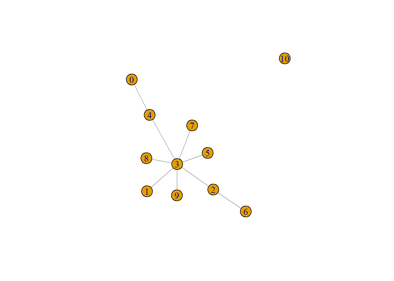
pseudo.og <- quickPseudotime(bcells_sce, use.dimred="PCA", outgroup=TRUE)
set.seed(10101)
plot(pseudo.og$mst)
pseudo.mnn <- quickPseudotime(bcells_sce, use.dimred="PCA", dist.method="mnn")
mnn.pseudo <- averagePseudotime(pseudo.mnn$ordering)
plotUMAP(bcells_sce, colour_by=I(mnn.pseudo), text_by="label", text_colour="red") +
    geom_line(data=pseudo.mnn$connected$UMAP, mapping=aes(x=UMAP_1, y=UMAP_2, group=edge))
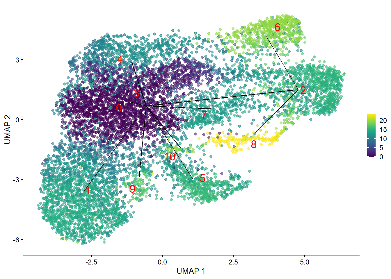
Now, let’s characterize these trajectories. We’ll identify differentially expressed genes along each path, providing a window into the cellular processes occurring within the B cells.
library(TSCAN)
pseudo <- testPseudotime(bcells_sce, pseudotime=tscan.pseudo[,1])[[1]]
pseudo$SYMBOL <- rowData(bcells_sce)$SYMBOL
pseudo[order(pseudo$p.value),]
## DataFrame with 21464 rows and 3 columns
##                  logFC   p.value       FDR
##              <numeric> <numeric> <numeric>
## PRG4       -0.12904766         0         0
## IGKC       -0.00925387         0         0
## FN1        -0.08238218         0         0
## CD74        0.11759914         0         0
## HLA-DRA     0.14591367         0         0
## ...                ...       ...       ...
## AC004264.1           0       NaN       NaN
## Z99756.1             0       NaN       NaN
## SCO2                 0       NaN       NaN
## AP001172.1           0       NaN       NaN
## CYYR1-AS1            0       NaN       NaN
# Making a copy of our SCE and including the pseudotimes in the colData.
bcells_sce2 <- bcells_sce
bcells_sce2$TSCAN.first <- pathStat(tscan.pseudo)[,1]
bcells_sce2$TSCAN.second <- pathStat(tscan.pseudo)[,2]
bcells_sce2$TSCAN.third <- pathStat(tscan.pseudo)[,3]
bcells_sce2$TSCAN.fourth <- pathStat(tscan.pseudo)[,4]
bcells_sce2$TSCAN.fifth <- pathStat(tscan.pseudo)[,5]

# Discarding cluster 10
discard <- "10"
keep <- colLabels(bcells_sce)!=discard
bcells_sce2 <- bcells_sce2[,keep]

# Testing against the first path again.
pseudo <- testPseudotime(bcells_sce2, pseudotime=bcells_sce2$TSCAN.first)


#this needs to change for plot expression
pseudo$SYMBOL <- rowData(bcells_sce2)$SYMBOL
sorted <- pseudo[order(pseudo$p.value),]

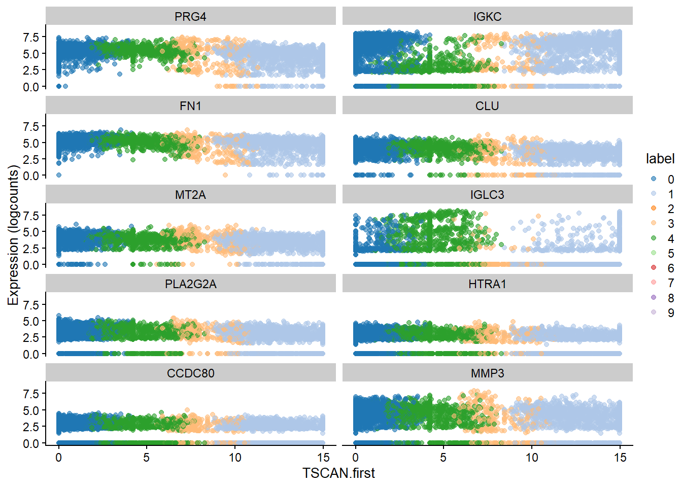
up.left <- sorted[sorted$logFC < 0,]
head(up.left, 10)
## DataFrame with 10 rows and 3 columns
##               logFC      p.value          FDR
##           <numeric>    <numeric>    <numeric>
## PRG4    -0.12904766  0.00000e+00  0.00000e+00
## IGKC    -0.00925387  0.00000e+00  0.00000e+00
## FN1     -0.08238218  0.00000e+00  0.00000e+00
## CLU     -0.12507122  0.00000e+00  0.00000e+00
## MT2A    -0.10252680  0.00000e+00  0.00000e+00
## IGLC3   -0.00348289  0.00000e+00  0.00000e+00
## PLA2G2A -0.10827726 5.45969e-266 8.61995e-263
## HTRA1   -0.10037404 2.28873e-221 2.28222e-218
## CCDC80  -0.09213947 1.15077e-194 8.38556e-192
## MMP3    -0.11502285 7.57552e-180 4.94916e-177
up.left$SYMBOL = rownames(up.left)
best <- head(up.left$SYMBOL, 10)

plotExpression(bcells_sce2, features=best,
    x="TSCAN.first", colour_by="label")#
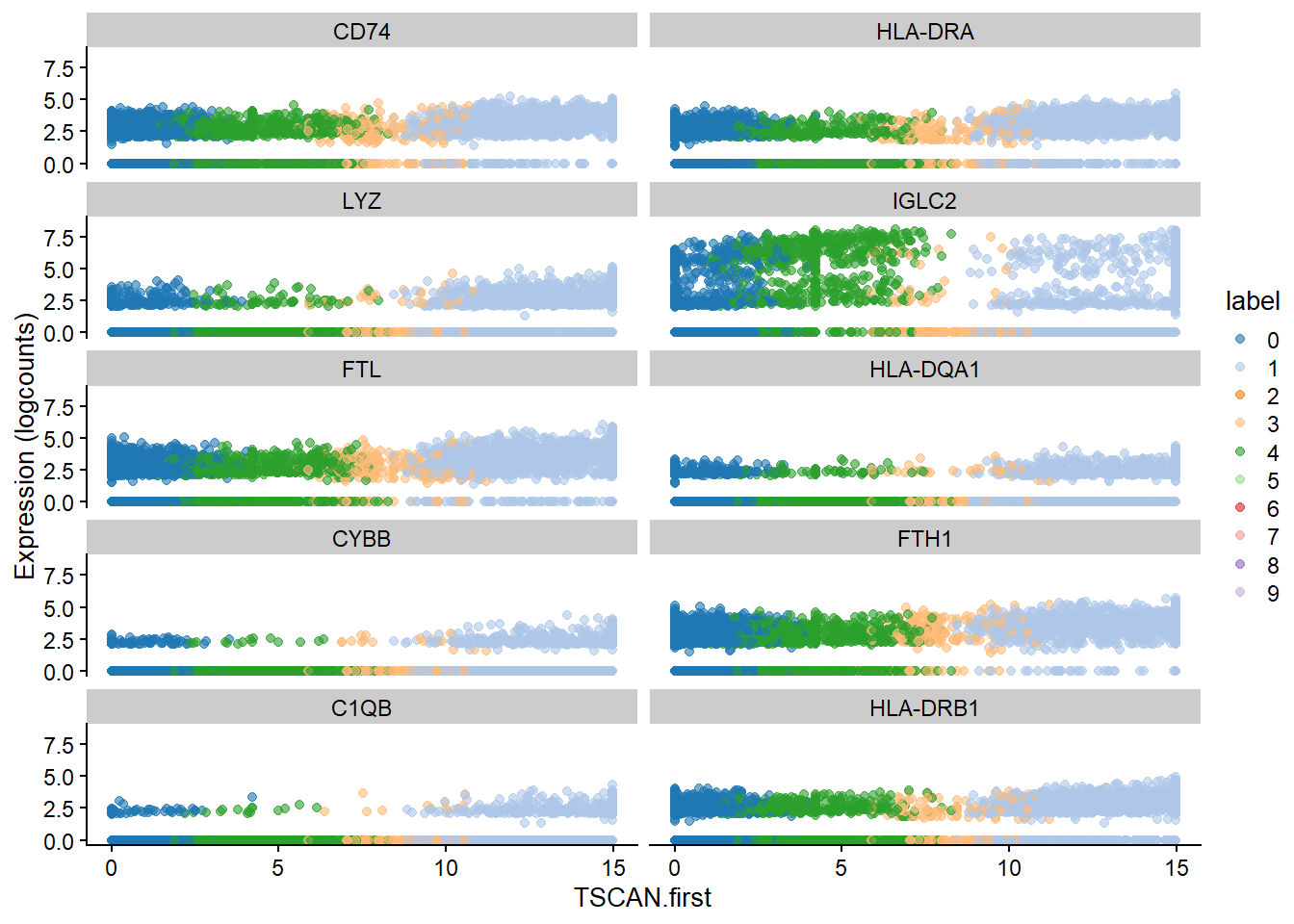
up.right <- sorted[sorted$logFC > 0,]
head(up.right, 10)
## DataFrame with 10 rows and 3 columns
##               logFC      p.value          FDR
##           <numeric>    <numeric>    <numeric>
## CD74     0.11759914  0.00000e+00  0.00000e+00
## HLA-DRA  0.14591367  0.00000e+00  0.00000e+00
## LYZ      0.13306120  0.00000e+00  0.00000e+00
## IGLC2    0.00955358  0.00000e+00  0.00000e+00
## FTL      0.11057968 6.22904e-288 1.07287e-284
## HLA-DQA1 0.08043531 3.06229e-264 4.46294e-261
## CYBB     0.06261430 3.31455e-255 4.48553e-252
## FTH1     0.09286146 4.16170e-253 5.25650e-250
## C1QB     0.05828614 4.61523e-253 5.46501e-250
## HLA-DRB1 0.09385772 7.34657e-250 8.18753e-247
up.right$SYMBOL = rownames(up.right)
best <- head(up.right$SYMBOL, 10)
plotExpression(bcells_sce2, features=best,
    x="TSCAN.first", colour_by="label")
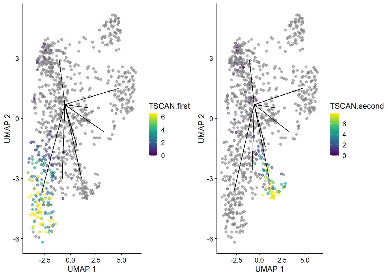
Finally, let’s explore trajectory change paths. These paths offer a glimpse into the dynamic changes occurring within the B-cell population, shedding light on their complex biology.
starter <- "3"
tscan.pseudo3 <- orderCells(map.tscan, mst, start=starter)
# Making a copy and giving the paths more friendly names.
sub.nest <- bcells_sce
sub.nest$TSCAN.first <- pathStat(tscan.pseudo3)[,1]
sub.nest$TSCAN.second <- pathStat(tscan.pseudo3)[,2]
sub.nest$TSCAN.third <- pathStat(tscan.pseudo3)[,3]
sub.nest$TSCAN.fourth <- pathStat(tscan.pseudo3)[,4]
sub.nest$TSCAN.fifth<- pathStat(tscan.pseudo3)[,5]
sub.nest$TSCAN.sixth <- pathStat(tscan.pseudo3)[,6]
sub.nest$TSCAN.seventh <- pathStat(tscan.pseudo3)[,7]
sub.nest$TSCAN.eighth <- pathStat(tscan.pseudo3)[,8]

# Subsetting to the desired cluster containing the branch point.
keep <- colLabels(bcells_sce2) == starter
sub.nest <- sub.nest[,keep]

# Showing only the lines to/from cluster 3 aka the star of the show
line.data.sub <- line.data[grepl("^3--", line.data$edge) | grepl("--3$", line.data$edge),]
ggline <- geom_line(data=line.data.sub, mapping=aes(x=UMAP_1, y=UMAP_2, group=edge))

gridExtra::grid.arrange(
    plotUMAP(sub.nest, colour_by="TSCAN.first") + ggline,
    plotUMAP(sub.nest, colour_by="TSCAN.second") + ggline,
    ncol=2
)
Conclusion
In delving into the intricate genetic makeup of arthritic B cells, our journey through scRNA-seq analysis has unveiled invaluable insights into genes that might influence the way b cells commit toa certain path in inflammatory arthritis. Of course, the exploration doesn’t end here; we could continue our analysis exploring ligand-receptor interactions between B cell clusters and other immune cell populations.
As we navigate through each trajectory mapped and gene characterized, we uncover layers of complexity within the immune system. These discoveries not only deepen our understanding of autoimmune diseases but also pave the way for breakthroughs that can be further explored in the laboratory to improve diagnostics and targeted therapies. With each revelation, we inch closer to deciphering the mysteries of autoimmune diseases and charting a course toward improved patient outcomes because in the pursuit of knowledge lies the promise of progress.