Insights from a Colon Cancer Trial

This analysis will be based on colon data from the survival package in R, representing valuable insights from an early successful trial of adjuvant chemotherapy for colon cancer. In this study, levamisole, known for its low toxicity, and 5-fluorouracil (5-FU), a moderately toxic chemotherapy agent, were administered.

Data validation and cleaning
This was the first step because analysis is easier when you understand the data structure and content.

library(survival)
library(tidyverse)
#examining data structure
c_data = colon
dim(c_data)
str(c_data)
head(c_data)
class(c_data)
as_tibble(c_data)

#data cleaning
#check for duplicate rows
unique(c_data) 
#remove rows with missing values 
c_data = na.omit(c_data)
# check for complete data (no missing values)
complete.cases(c_data)

#data summary
summary(c_data)
summary(c_data$age)
table(c_data$sex)
str(c_data)
c_data$timemn = c_data$time/30

# create new dataframes based on event type
c_recurrence = subset(c_data, etype == 1)
c_death = subset(c_data, etype == 2)

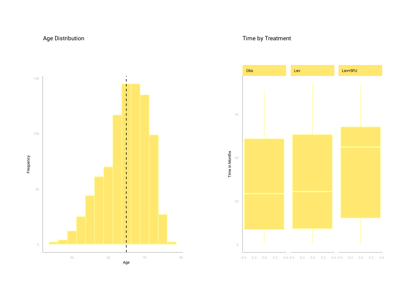
Seeing is believing, so it pays to plot the data as is. This process helps to pinpoint any potential outliers and provides insights into the fundamental structure of the data.

Data expRobototion lead to hypothesis testing:

Null Hypothesis (Ho) — There is no significant difference in the average (mean) survival times between the treatment groups are the same.

Alternative Hypothesis (Ha)— There is a significant difference in the treatment groups’ average (mean) survival times.

library(tidyverse)
library(ggpubr)
library(DescTools)


c_recurrence$rx = as.factor(c_recurrence$rx)
anova_model = aov(time ~ rx, data = c_recurrence)
summary(anova_model)
TukeyHSD (anova_model)

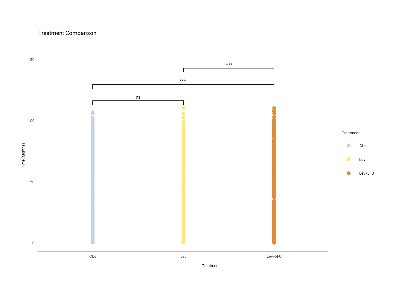
The ANOVA p. value (2.78e-05 ) indicates that the null hypothesis is to be rejected so this means I accept the alternative hypothesis. The Tukey HSD test provides more information with significant differences between ev+5FU-Obs (0.0000554) and Lev+5FU-Lev (0.0009525) and no significant difference between Lev-Obs (0.7826875).

Q: Is there a significant difference in the average (mean) survival times between male and female patients?

# Subset the dataset into male and female groups
male_group <- subset(c_death, sex == 1)
female_group <- subset(c_death, sex == 0)

# Perform an independent two-sample t-test
t_test_result <- t.test(male_group$time, female_group$time, paired = FALSE)

# Print the results
print(t_test_result)

Based on the provided results, there is no significant evidence to conclude that there is a difference in the average survival times between male and female patients.

Q: Is there a significant correlation between the number of nodes and time to recurrence?

#Calculate the correlation between "nodes" and "timemn"
cor.test(c_data$nodes, c_data$timemn)

Based on the results, there is a weak negative correlation between the number of nodes and time. As the number of nodes increases, the time in years tends to decrease. The p-value (< 2.2e-16) is almost zero, which suggests a strong level of confidence.

Linear regression could help you better understand the relationship of nodes and time to recurrence.

library(stats)
model <- lm(timemn ~ nodes, data = c_data)
summary(model)

Just to see how other models fit

#finding the best model
library(AICcmodavg)

#fit candidate models
model1 <- lm(timemn ~ age, data = c_data)
model2 <- lm(timemn ~ nodes, data = c_data)
model3 <- lm(timemn ~ age + nodes, data = c_data)
model4 <- lm(timemn ~ age * nodes, data = c_data)

models = list(model1, model2,model3, model4)
model_names = c("model1", "model2", "model3", "model4")
aictab(cand.set = models, modnames = model_names)

model 2 stands out as the best model with the lowest AICc value, the highest AICc weight, and the smallest Delta_AICc compared to the other models.

Survival Analysis

library(survival)
library(survminer)
library(ggthemes)

survival_object <- Surv(time = c_data$timemn, event = c_data$etype==2)

#Kaplan-Meier Survival Curve
km_fit <- survfit(survival_object ~ c_data$rx)
summary(km_fit)

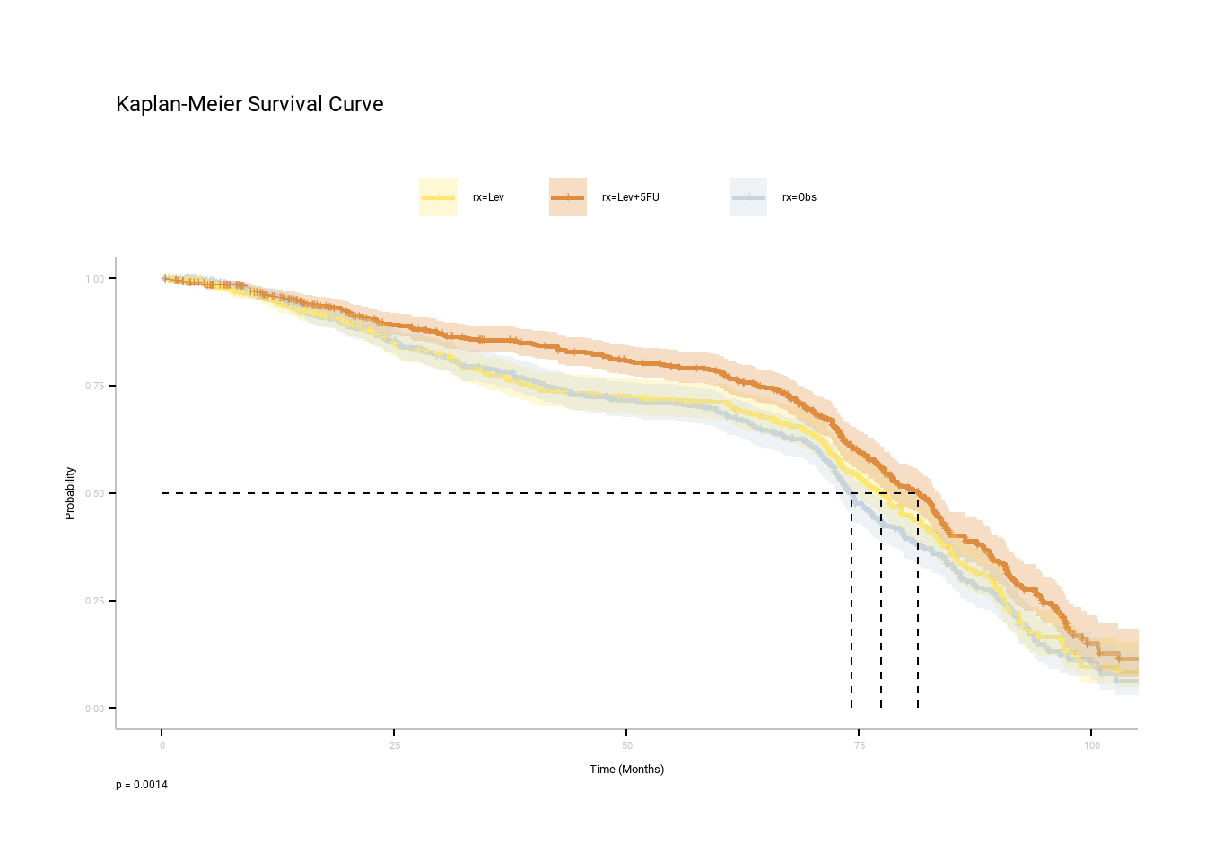
The curves for the three options are similar but Lev + 5FU has the highest median time of survival of 83.5 months.

In conclusion, this analysis has not only answered the fundamental question of treatment effectiveness but also satisfies curiosity, providing a comprehensive understanding of various factors influencing survival times in colon cancer patients.